Transactions on Machine Learning Research (TMLR), 2026

Stabilizing Consistency Training:
A Flow Map Analysis and Self-Distillation

Youngjoong Kim, Duhoe Kim, Woosung Kim, Jaesik Park†
Seoul National University
†Corresponding author
Figure 1. From consistency training to improved Self-Distillation. Consistency training learns a mapping over conditional velocity, often suffering from training instability and reproducibility issues. Relaxing the time condition mitigates this instability, and self-distillation aligns a target with the marginal velocity field. However, directly applying self-distillation leads to unstable training. We therefore reformulate the objective and incorporate classifier-free guidance (iSD-T), further stabilizing training and improving reproducibility.

Abstract

Consistency models have been proposed for fast generative modeling, achieving results competitive with diffusion and flow models. However, these methods exhibit instability and limited reproducibility when training from scratch, motivating subsequent work to explain and stabilize these issues. While these efforts have provided valuable insights, the explanations remain fragmented, and the theoretical relationships remain unclear. In this work, we provide a theoretical examination of consistency models by analyzing them from a flow map-based perspective. This joint analysis clarifies how training and convergence behavior can give rise to degenerate solutions. Building on these insights, we revisit self-distillation as a practical remedy for certain forms of suboptimal convergence. To avoid excessive gradient norms during its optimization, we reformulate its objective empirically, yielding improved Self-Distillation (iSD). We further extend iSD with training-time classifier-free guidance, yielding iSD-T, which improves performance and reproducibility in the studied settings. We demonstrate that iSD extends beyond image generation to diffusion-based policy learning, without reliance on pretrained diffusion models for initialization.

Section 3Preliminary

Flow Matching. Given a dataset \(X\) with underlying distribution \(p_X\), flow matching models are trained to match the velocity fields of continuous flows, starting from a tractable distribution \(p_Z\). Prior work constructs such flows via an interpolation, \(x_t = \alpha_tx + \sigma_t z\), where \(x\sim p_X\) and \(z\sim p_Z\). With the constructed flow, the flow matching models optimize the squared error between the conditional velocity \(v_t(x_t|x) = \alpha'_tx + \frac{\sigma'_t}{\sigma_t}(x_t - \alpha_tx)\) and a network \(F_\theta(x_t; t)\):

\[\mathcal L_\text{CFM} = \mathbb E_{x,z,t}\left[\|F_\theta(x_t; t) - v_t(x_t|x)\|^2_2\right],\qquad F_\theta(x_t; t)\approx v^*_t(x_t) = \mathbb E_{x|x_t}[v_t(x_t|x)].\]

Flow Map. From flows defined by interpolation, our goal is to draw samples from the target distribution in a few sampling steps. To this end, we adopt a flow map \(f(x_t; t, s)\), which is a mapping between two points \(x_t\) and \(x_s\ (s<t)\) on the same trajectory (Kim et al., 2024; Boffi et al., 2025):

\[f(x_t; t, s) = x_t + \int^s_tv_\tau^*(x_\tau)d\tau = x_s.\]

Training Flow Map. Since the flow map is defined as an integral, direct supervision from scratch is challenging. Recent studies adopt consistency training (Song et al., 2023) to avoid data generation, which can be derived from the Eulerian equation:

\[\partial_t f(x_t; t, s) + v^*_t(x_t)\cdot\nabla_xf(x_t; t, s) = 0.\]

To train a flow map network \(f_\theta(x_t; t, s)\) using this equation, Eulerian distillation (Boffi et al., 2025) formulates the objective as a squared minimization problem:

\[\mathcal L_\mathrm{ED} = \mathbb E_{x,z,t,s}\left[\|\partial_tf_\theta(x_t; t, s) + v^*_t(x_t)\cdot\nabla_xf_\theta(x_t; t, s)\|^2_2\right].\]

For consistency training from scratch, using \(v_t(x_t|x)\) instead of \(v^*_t(x_t)\) is a more common choice:

\[\mathcal L_\mathrm{CT} = \mathbb E\left[\left\|f_\theta(x_t; t, s) - \operatorname{sg}\left[f_\theta(x_t; t, s) - \left[\partial_tf_\theta(x_t; t, s) + {\color{#b4462b}v_t(x_t|x)}\cdot\nabla_xf_\theta(x_t; t, s)\right]\right]\right\|^2_2\right].\]

Since \(\mathcal L_\mathrm{ED}\) involves a Jacobian-vector product (JVP), its optimization requires second-order differentiation, introducing computational overhead. In contrast, consistency distillation \(\mathcal L_\mathrm{CD}\) and consistency training \(\mathcal L_\mathrm{CT}\) use a stop-gradient operation, avoiding this issue. However, they alter gradient dynamics, potentially affecting training stability.

Section 4

Analysis of Instability

In this section, we analyze instability and reproducibility in consistency models from a flow map perspective, focusing on how different design choices affect convergence properties and training dynamics. Based on this analysis, we explain why training from scratch may deviate from the desired flow map in practical settings.

4.1 Flow Map Representation for Analysis

To enable a systematic analysis of training instability in consistency models, we propose a flow map representation for commonly used interpolations, expressed as a one-step Euler solution with a network \(F_\theta\):

\[f_\theta(x_t; t, s) = \nu^{-1}(A_{t,s}'x_t - A_{t,s}F_\theta(x_t; t, s)),\qquad A_{t,s}=\sigma_t\alpha_s - \sigma_s\alpha_t.\]

Proposition 4.1 (Interpretation of Recent Methods)

The methods listed in Table 1 can be interpreted within the flow map representation, satisfying the following transport equation:

\[\partial_tf_\theta(x_t; t, s) + \tau_t(x_t, x)\cdot\nabla_xf_\theta(x_t; t, s) = 0,\]

where \(x_t\) is given by the Interpolant, \(\tau_t\) by the Trajectory, and \(t, s\) by the Timestep, as summarized in Table 1.

ModelInterpolant \(x_t\)Trajectory \(\tau_t\)TimestepJVPObjective
Distillation-based Methods
FMM-EMDAny (Linear)\(\Phi_t(x_t)\)\(s < t\)Exact\(\mathcal L_\mathrm{ED}\)
AYF-EMDAny (Linear)\(\Phi_t(x_t)\)\(s < t\)Exact\(\mathcal L_\mathrm{CD}\)
sCDTrigonometric\(\Phi_t(x_t)\)\(s=0\)Exact\(\mathcal L_\mathrm{CD}\)
Consistency Training Methods
MeanFlowLinear\(v_t(x_t|x)\)\(s < t\)Exact\(\mathcal L_\mathrm{CT}\)
ConsistencyFMLinear\(v_t(x_t|x)\)\(s=0\)Approx.\(\mathcal L_\mathrm{CT}\)
sCTTrigonometric\(v_t(x_t|x)\)\(s=0\)Exact\(\mathcal L_\mathrm{CT}\)
UCGMAny (Linear, Trig.)\(v_t(x_t|x)\)\(s=0\)Approx.\(\mathcal L_\mathrm{CT}\)
Self-Distillation Methods
Shortcut ModelLinear\(F_\theta(x_t; t, t)\)\(s < t\)Approx.\(\mathcal L_\text{SD}\)
ESDAny (Linear)\(F_\theta(x_t; t, t)\)\(s < t\)Exact\(\mathcal L_\mathrm{SD}\)
iSD (Ours)Any (Linear, Trig.)\(F_\theta(x_t; t, t)\)\(s < t\)Approx.\(\mathcal L_\mathrm{SD\text{-}R}\)

Table 1. Summary of recent consistency models interpreted under the flow map representation. Interpolants in parentheses denote settings realized in the cited work. \(\Phi_t(x_t)\) is the teacher network and \(F_\theta(x_t; t, s)\) is the training network. Our method is aligned with the learned marginal velocity \(F_\theta(x_t; t, t)\) and the relaxed time condition \(s<t\), while reformulating Eulerian self-distillation (ESD) to reduce the gradient norm problem.

4.2 Suboptimality and Instability

Guidance Velocity

Most consistency training approaches are guided by a conditional velocity. However, this setup can contribute to training instability. To examine its effect, we consider Eulerian distillation with a conditional velocity field. Following Boffi et al. (2025), we refer to this as direct training.

\[\mathcal L_\mathrm{DT} = \mathbb E\left[\|\partial_tf_{\theta}(x_t; t, s) + {\color{#b4462b}v_t(x_t|x)}\cdot\nabla_xf_{\theta}(x_t; t, s)\|^2_2\right].\]

Since the global optimum of Eulerian distillation corresponds to the flow map, we show that direct training does not guarantee convergence to this solution by comparing their stationary conditions.

Proposition 4.2 (Stationary Condition of Direct Training)

A stationary point of direct training satisfies

\[\mathcal S_\mathrm{DT} = \mathcal S_\mathrm{ED} + {\color{#b4462b}C} = 0,\quad {\color{#b4462b}C = \nabla\cdot(\rho_t\Sigma_{\Delta v|x_t}\nabla_x f_\theta)},\]

where \(\mathcal S_\mathrm{ED}\) is the stationary condition of Eulerian distillation, \(\Delta v = v_t(x_t|x) - v^*_t(x_t)\), and \(\Sigma_{\Delta v|x_t}\) is the conditional covariance \(\mathrm{Cov}_{x|x_t}[\Delta v]\). This follows from applying the Euler-Lagrange equation to \(\mathcal L_\mathrm{DT}\). This suggests that training can admit a degenerate flow map (\(\mathcal S_\mathrm{ED} = -C\ne 0\)), which is a suboptimal solution.

Thus, the discrepancy is not only an objective-level mismatch: through the term \(C\), it can actually shift the stationary point and admit degenerate flow maps. This term arises from the gap \(\Delta v\) between the marginal velocity \(v^*_t(x_t)\) and the per-sample conditional velocity \(v_t(x_t|x)\).

\(\mathcal L_\mathrm{DT}\)
\(\mathcal L_\mathrm{ED}\)
Ground truth
Figure 2. Toy experiments with a 5-layer MLP (batch size of 2048). \(\mathcal L_\mathrm{DT}\) drives flow map training toward a suboptimal solution, while \(\mathcal L_\mathrm{ED}\) leads to a solution close to the ground truth.

Compared to Eulerian distillation, which successfully learns the ground-truth distribution, direct training converges to a degenerate distribution, consistent with the proposition.

When a stop-gradient operation is applied to \(\mathcal L_\mathrm{DT}\), it coincides with the consistency training objective \(\mathcal L_\mathrm{CT}\). This objective can recover solutions satisfying the Eulerian equation, even when guided by conditional velocity. However, this holds only at the expectation level, and a small batch size can induce a residual gap.

Proposition 4.3 (Expectation-level Realization of Consistency Training)

Let \(L_*f_\theta=\partial_t f_\theta+v_t^*\cdot\nabla_x f_\theta\) denote the Eulerian operator applied to \(f_\theta\). The stationary condition of consistency training is

\[\mathcal S_\mathrm{CT} = L_*f_\theta + {\color{#b4462b}\mathbb E_{x|x_t}[\Delta v\cdot\nabla_x f_\theta]} = 0,\]

when \(\rho_t > 0\). This admits the desired flow map as a fixed-point solution, \(L_*f_\theta = 0\), since the second term vanishes by \(\mathbb E_{x|x_t}[\Delta v] = 0\) in expectation. However, under finite-batch estimation, the empirical residual induced by \(\Delta v\) may remain, which can perturb the fixed-point training dynamics.

\(\mathcal L_\mathrm{CT}\)
\(\mathcal L_\mathrm{ED}\)
\(B=2048\)
\(B=512\)
\(B=128\)

\(\mathcal L_\mathrm{ED}\) over training steps.

Figure 3. (Left) Consistency training \(\mathcal L_\mathrm{CT}\) exhibits drift toward degenerate distributions as the batch size \(B\) decreases. (Right) Estimating the optimality of flow maps using \(\mathcal L_\mathrm{ED}\). Solid lines indicate a batch size of 2048, and dash-dot lines indicate 128.

Figure 3 shows drift toward a degenerate solution as the batch size decreases, which is consistent with the finite-batch residual in Proposition 4.3. We also measure \(\mathcal L_\mathrm{ED}\) for the toy dataset, which serves as a proxy for estimating the optimality of flow maps. While it does not fully reflect generation performance, consistency training with small batch sizes and direct training yield higher \(\mathcal L_\mathrm{ED}\) values, which can be interpreted as a signal of a degenerate solution.

From this perspective, both the bias term in Proposition 4.2 and the finite-batch residual in Proposition 4.3 originate from the same conditional-marginal velocity mismatch. We therefore consider incorporating the marginal velocity as the underlying flow field to reduce this gap in the next section.

AppendixDirect intervention & batch size on ImageNet
\[v^\gamma_t(x_t) = (1-\gamma)v^*_t(x_t) + \gamma v_t(x_t|x)\]
\(\gamma\)1.000.750.500.250.00
\(\mathcal L_\mathrm{ED}\)0.340.240.170.120.10
\(\mathcal L_\mathrm{CT}\)0.160.150.150.120.10

\(\mathcal L_\mathrm{ED}\) in toy experiments

\(\gamma\)1.00.50.0
FID120.49112.42110.38
\(\sigma\)204.0792.4361.94

FID and \(\sigma\) in ablation settings

Table 10. Direct intervention on guiding velocity by interpolating marginal velocity (\(\gamma=0\)) and conditional velocity (\(\gamma=1\)). The marginal velocity guidance shows lower FID and lower loss variance. This provides empirical evidence consistent with the view: the gradient difference induced by the guiding velocity can affect optimization and is associated with suboptimality and instability.

Weight Initializations

We further observe that consistency models with \(s=0\) are sensitive to weight initialization, which can affect reproducibility. Recent approaches rely on initialization with pretrained flow models, where the network is already approximately aligned with target flows. This reduces certain early-stage instability, and is often referred to as a preconditioner (Geng et al., 2025). We find that performance varies with the preconditioner, and reproducing results without known preconditioners can be challenging.

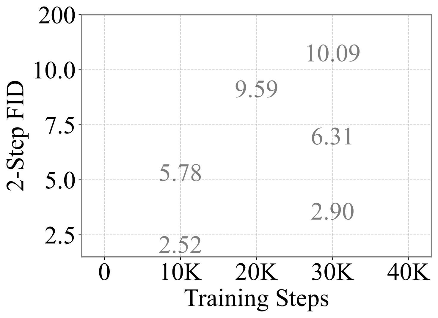
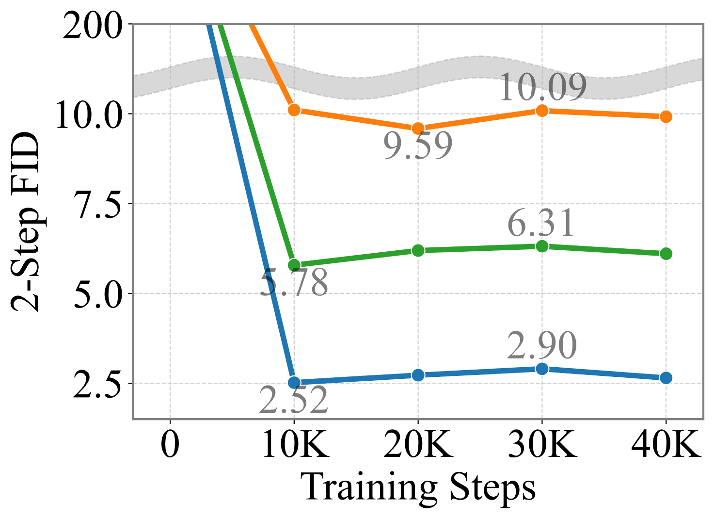
PreconditionerPreconditioner FID↓2-FID↓
Multistep Baseline1.21 (UCGM-S, 30-step)2.52
LightningDiT2.17 (Euler, 250-step)9.59
In-house Flow Model2.41 (UCGM-S, 30-step)5.78
w/o Preconditioner-419.60
Reported Baseline1.21 (UCGM-S, 30-step)1.42

Table 2. Consistency training results under different preconditioners. Preconditioner FID denotes the FIDs of pretrained networks for given ODE solver and sampling-step pairs. 2-FID denotes two-step FIDs of consistency models initialized from the corresponding preconditioner.

We evaluated an open-source consistency model (Sun et al., 2025) on ImageNet-1K \(256\!\times\!256\). With the baseline preconditioner, the model achieves reasonable results but remains above the reported FID. However, with other pretrained flow models, the FIDs become worse.

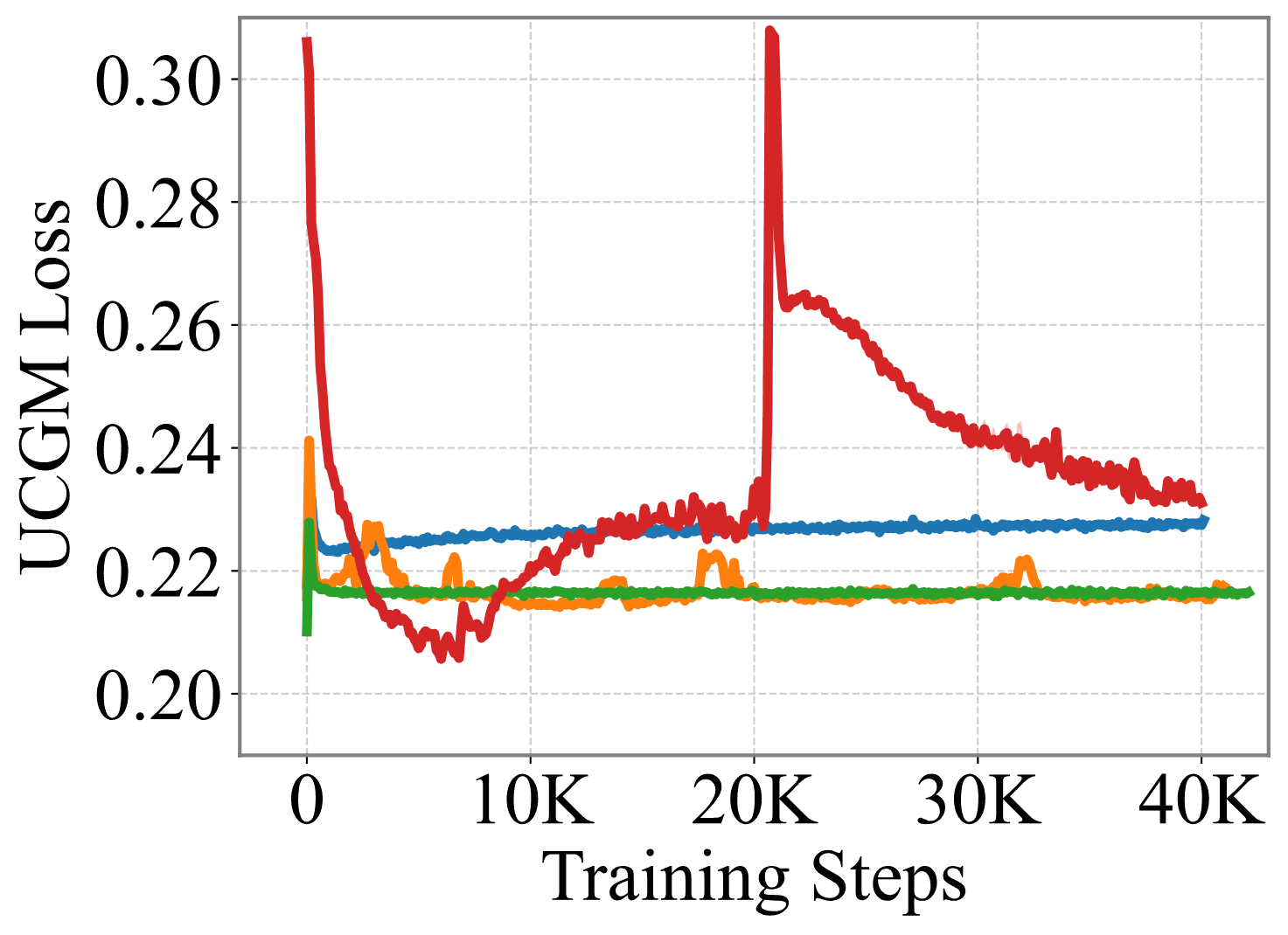
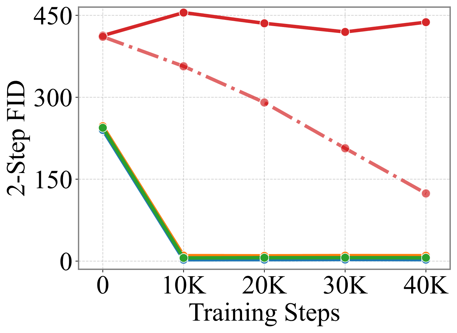
The resulting few-step FIDs are inconsistent: stronger preconditioners do not necessarily yield better consistency models. Additionally, models diverge when initialized randomly, suggesting that the optimum is inaccessible in this case.

As a complementary hypothesis, this can be understood from the stop-gradient (fixed-point) updates of consistency models: initialization matters as training is driven toward nearby fixed points rather than the global optimum. The result suggests the possible existence of attracting basins under different initialization weights.

AppendixTraining curves of consistency training
Training loss over training steps Two-step FIDs over training steps Rescaled two-step FIDs with a preconditioner
Legend: CT with baseline, LightningDiT, reproduced, and random initialization

Figure 9. (a) Training loss over training steps. (b) Two-step FIDs over training steps. (c) Rescaled Y-axis for the consistency model with a preconditioner. These results suggest that consistency training can be sensitive to initialization and the choice of preconditioner.

Time Condition

Some studies (Geng et al., 2025; Frans et al., 2025) enable training from scratch without a preconditioner. The key difference is that they allow \(s<t\), while others fix \(s=0\). Intuitively, training long-range mappings is more challenging than short-range ones. Under the flow map representation, Eulerian distillation can be written as

\[\mathcal L_\mathrm{ED} = \mathbb E\left[\left\|{\color{#7a838e}A''_{t,s}x_t} + {\color{#0070c0}A'_{t,s}(v^*_t - F_\theta)} - {\color{#b4462b}A_{t,s}\frac{dF_\theta}{dt}}\right\|^2_2\right] = \mathbb E\left[\left\|{\color{#0070c0}v^*_t - F_\theta} - {\color{#b4462b}(t - s)\frac{dF_\theta}{dt}}\right\|^2_2\right].\]
\(\alpha_t = 1-t,\ \sigma_t = t,\ t\in[0,1]\)
\(A''_{t,s}\)
\(A'_{t,s}\)
\(A_{t,s}\)

We observe that \(s\to t\) amplifies the flow matching term \(v^*_t - F_\theta\) since \(A''_{t,t}=A_{t,t}=0\), while \(s\to 0\) amplifies the linearization term involving the JVP \(dF_\theta/dt\). As the JVP is structurally more complex, we hypothesize that it may give rise to more undesired fixed points. This suggests that fixing \(s=0\) makes optimization less stable, while relaxing to \(s<t\) balances the terms and mitigates instability.

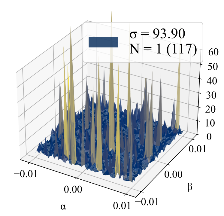
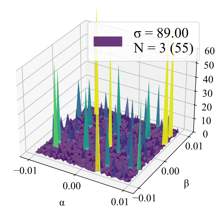
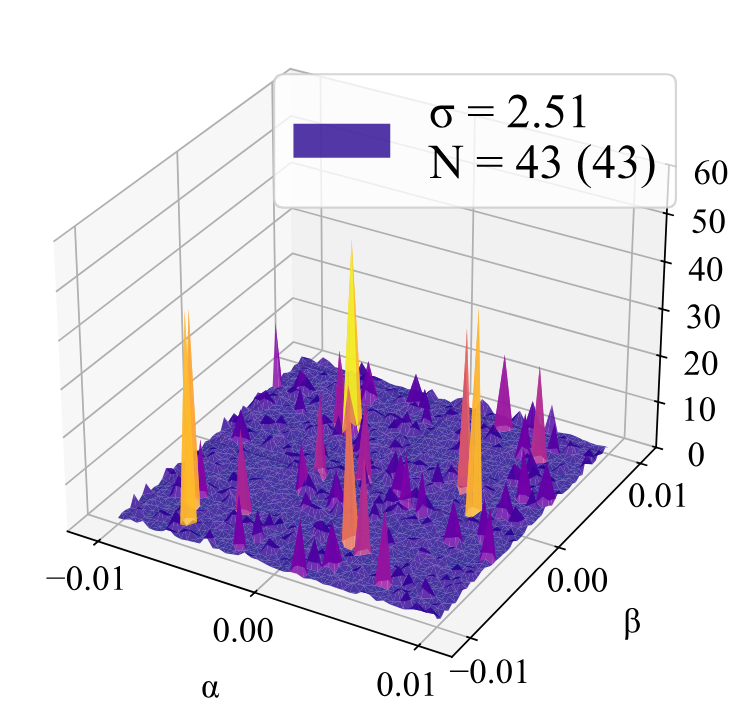
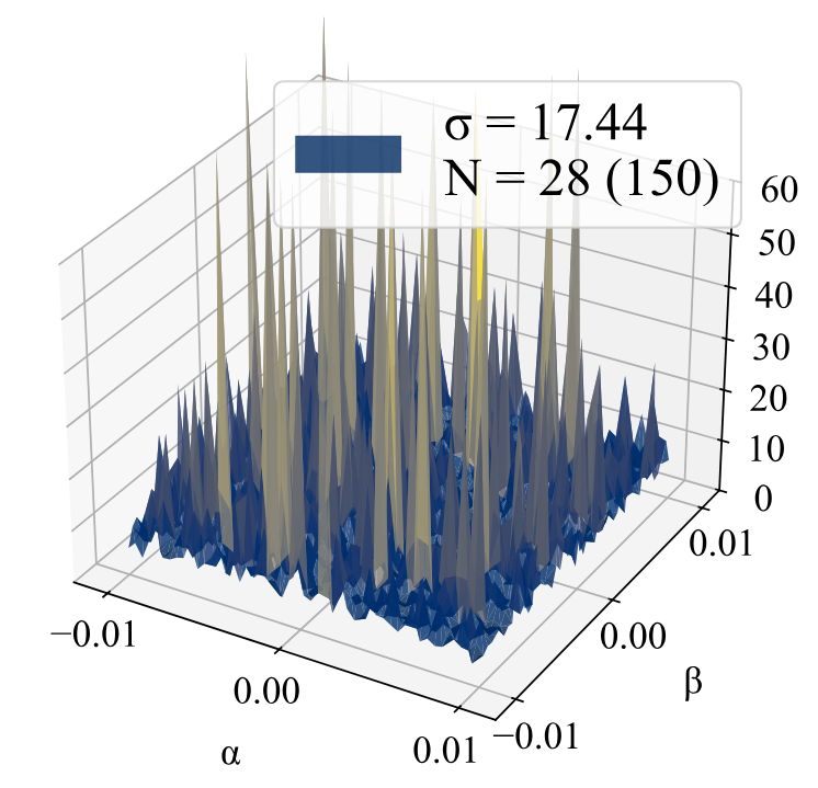
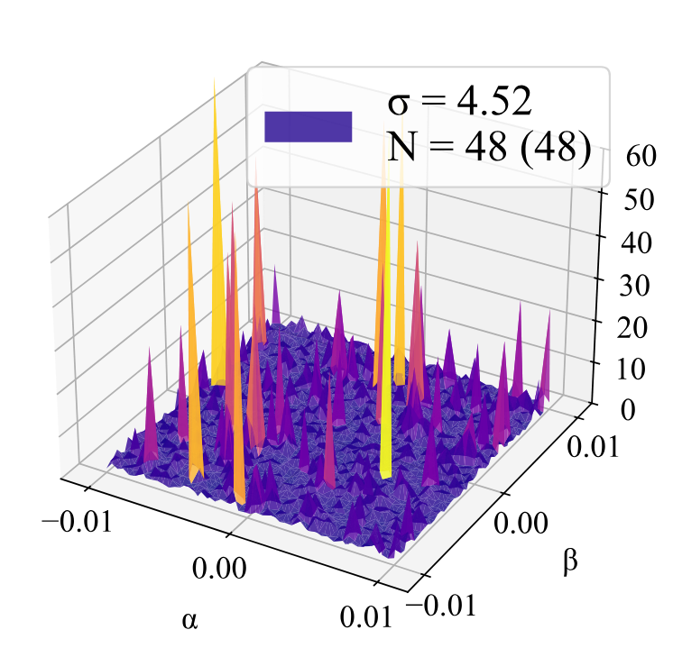
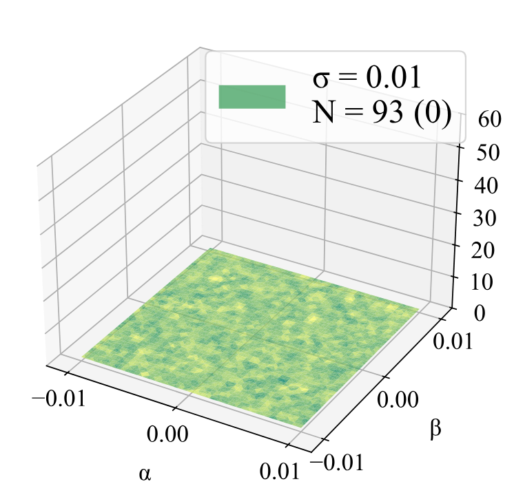
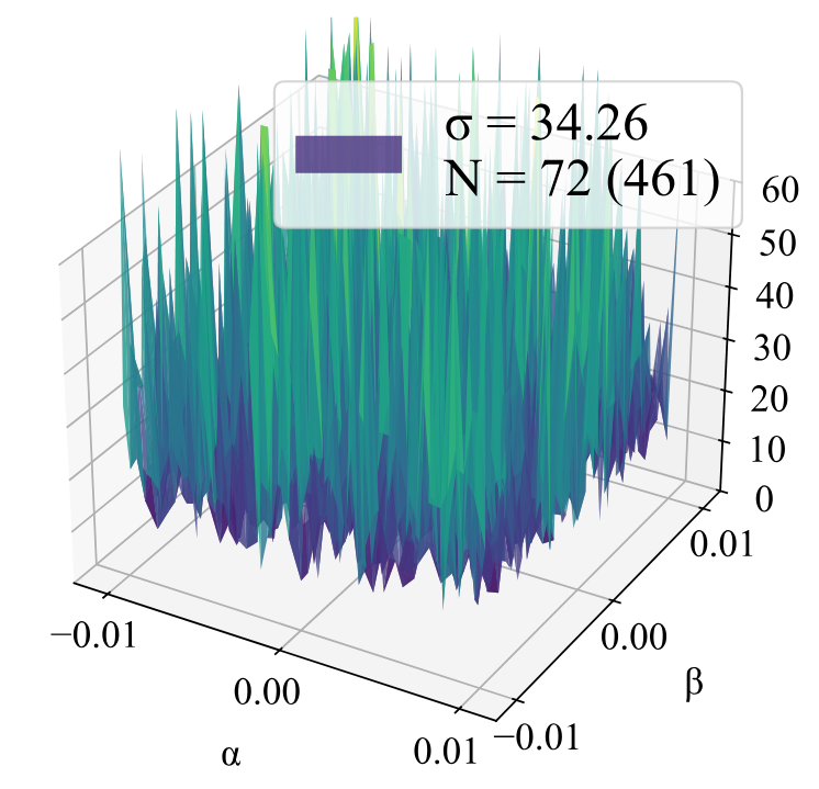
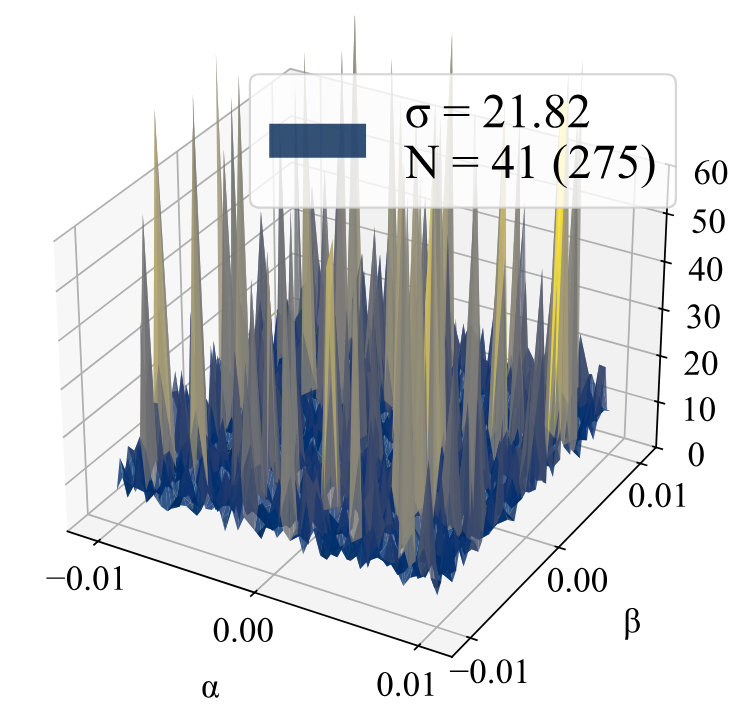
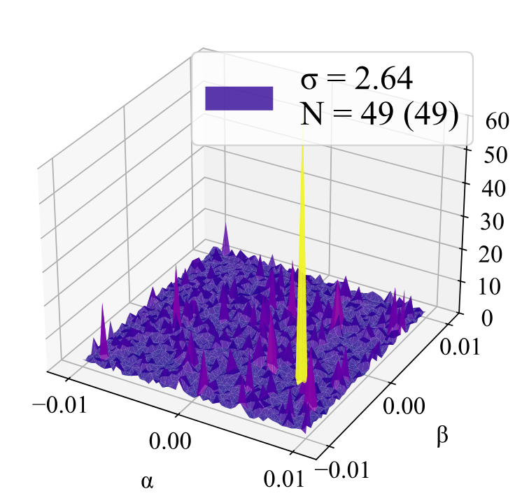
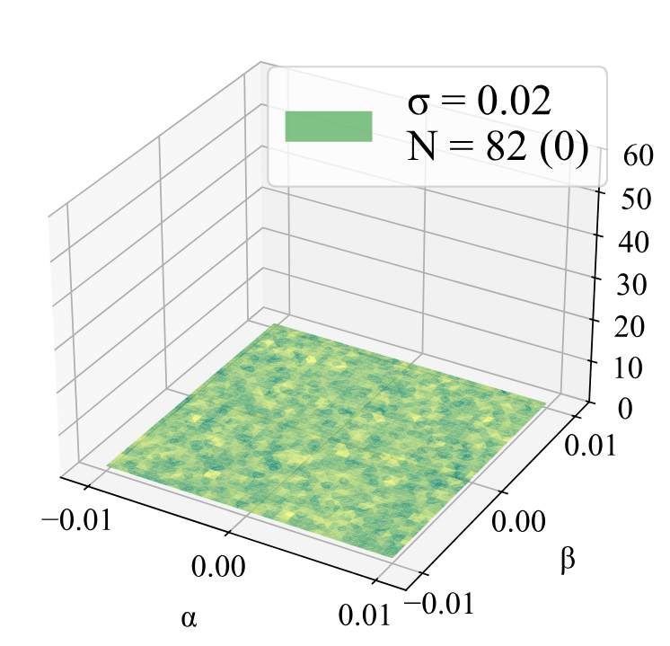
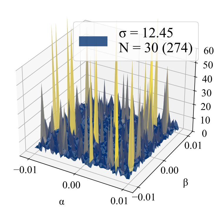
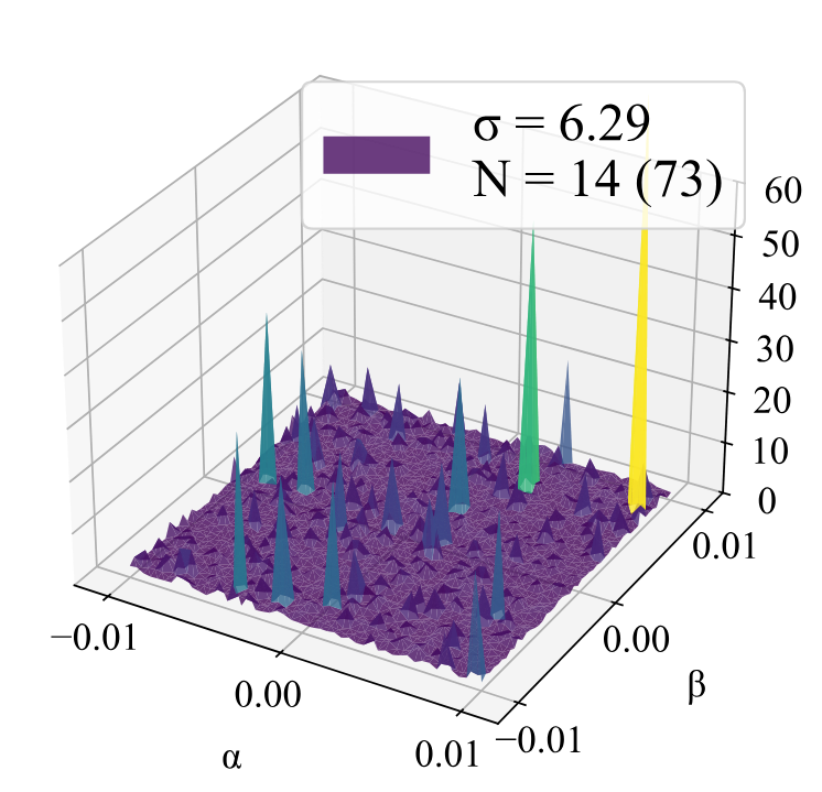
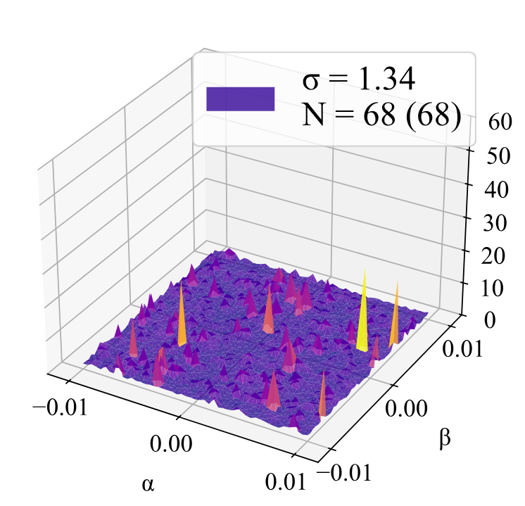
To support our hypothesis, we examine the loss landscapes of each objective, using their variance and number of spikes as proxies for training stability.
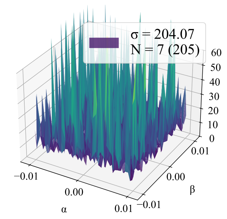
Loss landscape of the consistency modelConsistency Model
Loss landscape with time relaxationTime Relaxation
Loss landscape of self-distillation (ESD)Self-Distillation (ESD)
Loss landscape of iSDiSD (Ours)

Figure 4. Loss landscapes of four methods. The standard deviation \(\sigma\) and the number of spikes \(N\) serve as diagnostic proxies for training stability. iSD shows lower variance and fewer spikes under the common reference range. \(\alpha\) and \(\beta\) denote the top-2 eigenvectors of the Hessian on ImageNet-1K with DiT-B/4. \(N\) denotes the number of samples outside each method's own empirical 95% range. Values in parentheses report the number of samples exceeding the range defined by iSD, as a common reference.

Time relaxation reduces loss variance and spikes, which can be interpreted as reduced risk of training divergence, supporting our claim. We also note that our method in the next section, iSD, produces even smoother landscapes.

AppendixStep size ablation
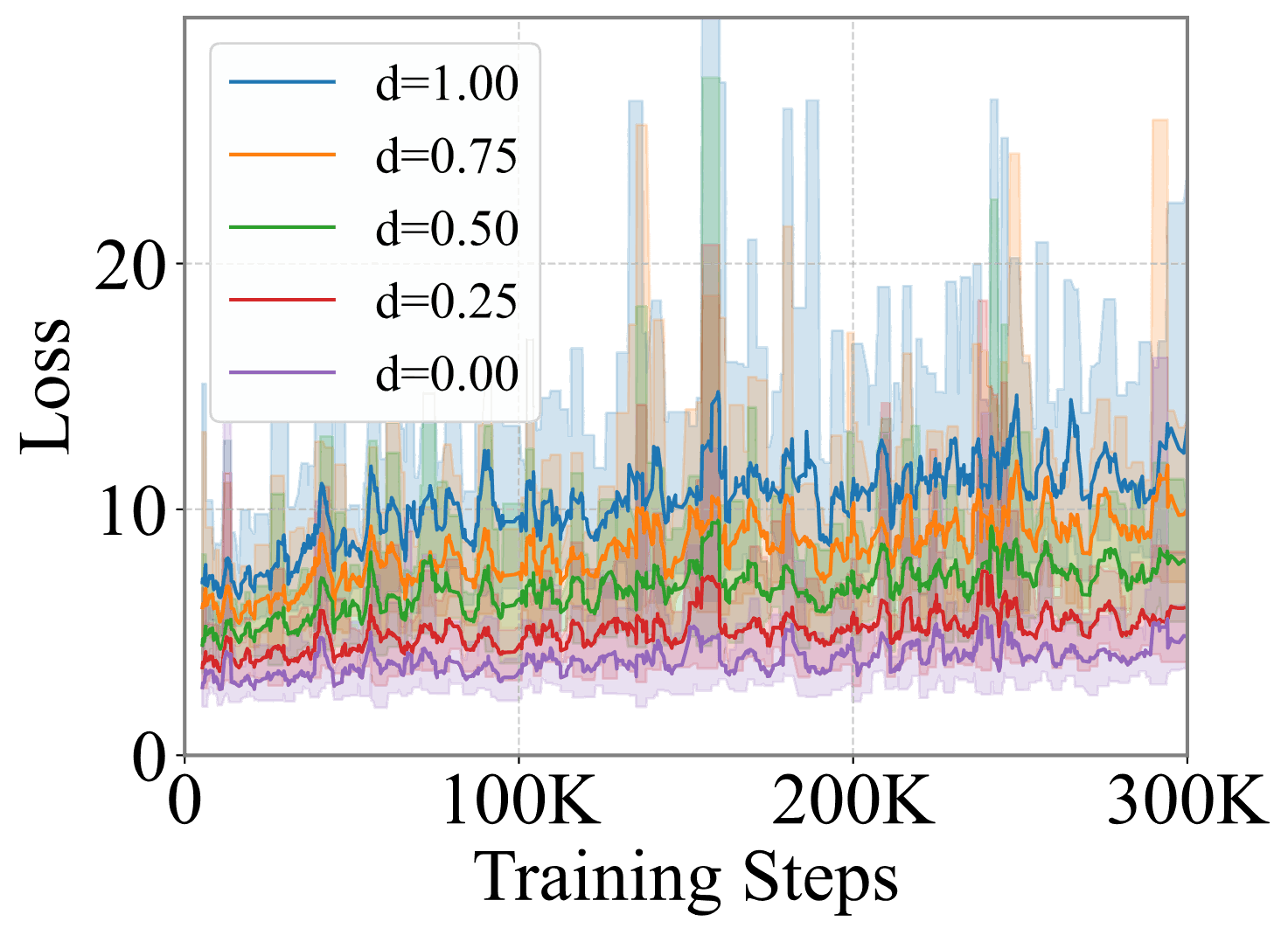
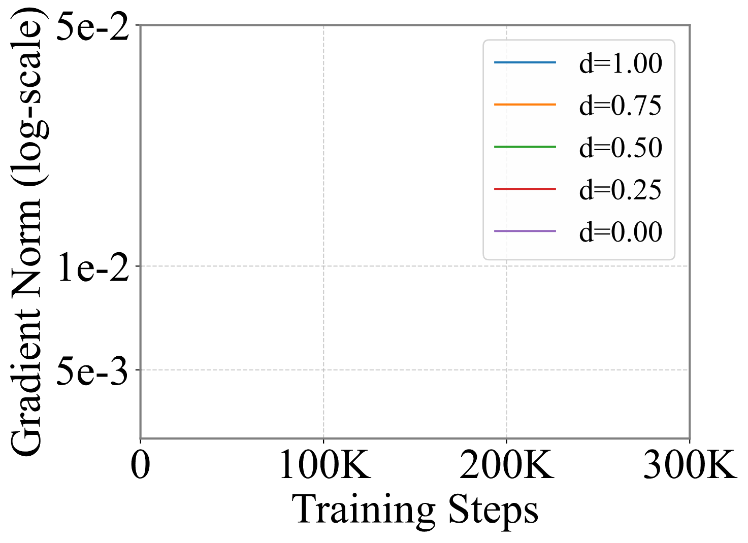
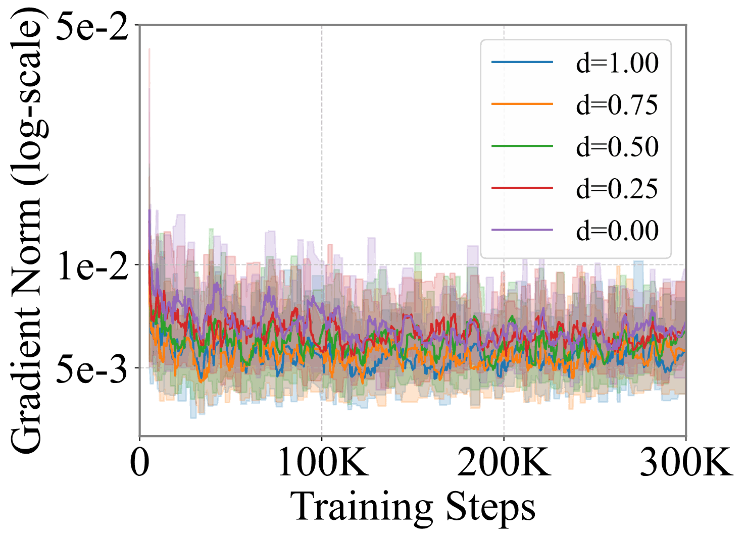
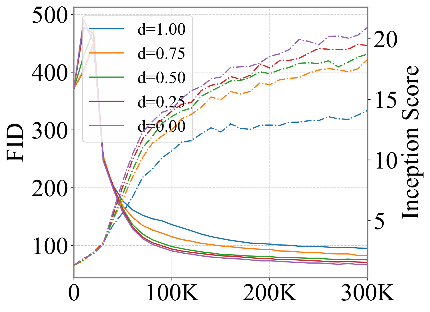
\[s = u\cdot \max\{t - d, 0\},\quad t\sim \mathrm{Beta}(0.8, 1.0),\quad u\sim \mathcal U[0, 1)\]
Loss over training steps across step size d Gradient norm across step size d FID and IS across step size d

Figure 11. \(d=0\) recovers the relaxed time condition \(s<t\), whereas \(d=1\) recovers fixed \(s=0\). Smaller \(d\) values are associated with lower loss values and better quantitative metrics in this setting. We note that these results are limited to a single-seed evaluation.

Summary

Consistency training admits the desired flow map only in expectation due to conditional velocity guidance, and small batches can introduce a non-vanishing empirical residual. We observe that performance is sensitive to weight initialization, which can be attributed to fixed-point updates. Time-condition relaxation is associated with training stability and can enable random weight initialization, contributing to reproducibility.

These mechanisms provide an explanation for limited stability and reproducibility across initializations and training settings. Motivated by this observation, we seek to improve them by eliminating reliance on preconditioners through time-condition relaxation and reducing this residual via marginal velocity guidance.
Section 5

Method

From Table 1, we identify that Eulerian Self-Distillation (ESD; Boffi et al., 2025) uses marginal velocity under a relaxed time condition. This can make random initialization feasible and reduce reliance on preconditioners. However, ESD exhibits large gradient norms on high-dimensional data, destabilizing training.

Since ESD is not intended to explicitly address the gradient norm problem, we reformulate self-distillation following the consistency-based formulation of Sabour et al. (2025). While this is an empirical optimization fix rather than a direct implication of Propositions 4.2 and 4.3, we observe that this can reduce gradient norms. We call this approach improved Self-Distillation (iSD).

5.1 improved Self-Distillation (iSD)

Eulerian Self-Distillation (ESD) jointly trains \(F_\theta(x_t; t, t)\) via flow matching and \(f_\theta(x_t; t, s)\) via Eulerian distillation, guided by its own velocity:

\[\mathcal L_\mathrm{SD} = \mathbb E\left[\|\partial_tf_{\theta}(x_t; t, s) + {\color{#0070c0}F_\theta(x_t; t, t)}\cdot\nabla_xf_\theta(x_t; t, s)\|^2_2\right].\]

Compared to direct training, this utilizes the model-induced marginal velocity \(v^*_t(x_t)\approx F_\theta(x_t; t, t)\) instead of the per-sample conditional velocity \(v_t(x_t|x)\), without requiring teacher networks. This encourages convergence to the marginal flow map and addresses suboptimality in Proposition 4.2.

Reformulation. To enable ESD while incorporating design choices, we propose to reformulate self-distillation \(\mathcal L_\mathrm{SD}\) using the flow map representation. In this case, the guidance velocity \(v_\theta(x_t; t) = F_\theta(x_t; t, t)\) corresponds to the marginal velocity under joint training of flow matching:

\[\mathcal L_\mathrm{SD} = \mathbb E\left[\left\| A''_{t,s}x_t + A'_{t,s}(v_\theta(x_t; t) - F_\theta(x_t; t, s)) - A_{t,s}\frac{dF_\theta(x_t; t, s)}{dt}\right\|^2_2\right].\]

To reduce gradient norms, we consider two stop-gradient placements: only the spatial derivative and the full derivative. Both yield theoretically well-defined objectives admitting the desired fixed points, and we empirically select the latter for lower gradient norm and computational efficiency:

\[\mathcal L_\mathrm{SD\text{-}R} = \mathbb E\left[\|F_\theta(x_t; t, s) - \operatorname{sg}\left[F_\mathrm{tgt}\right]\|^2_2\right],\quad F_\mathrm{tgt} = F_\theta + A''_{t,s}x_t + A'_{t,s}(v_\theta - F_\theta) - A_{t,s}\frac{dF_\theta}{dt}.\]
AppendixGradient norms of each method

Toy setting

ImageNet ablation setting (Linear, Pre-CFG 5.0)

Figure 8. Gradient norms of each method. The colored regions indicate 1 standard deviation. SD denotes Eulerian self-distillation (ESD), SD w/SG denotes the stop-gradient version of ESD introduced by Boffi et al. (2025), CT denotes consistency training, and iSD denotes our improved Self-Distillation.Toy curves are from the same re-run as the toy figures.

Thus, our final objective of improved Self-Distillation follows:

\[\mathcal L_\mathrm{iSD} = \lambda_1\mathcal L_\mathrm{CFM} + \lambda_2\mathcal L_\mathrm{SD\text{-}R},\qquad \mathcal L_\mathrm{CFM} = \mathbb E[\|F_\theta(x_t; t, t) - v_t(x_t|x)\|^2_2].\]

Consistency training can be viewed as a coupled fixed-point iteration with a parameterized target, whose contraction and global convergence are difficult to establish without additional assumptions. Instead, Appendix B.1 suggests that the objectives are aligned and non-conflicting. We leave contraction and global convergence properties for future work.

AppendixComparison with LSD & PSD
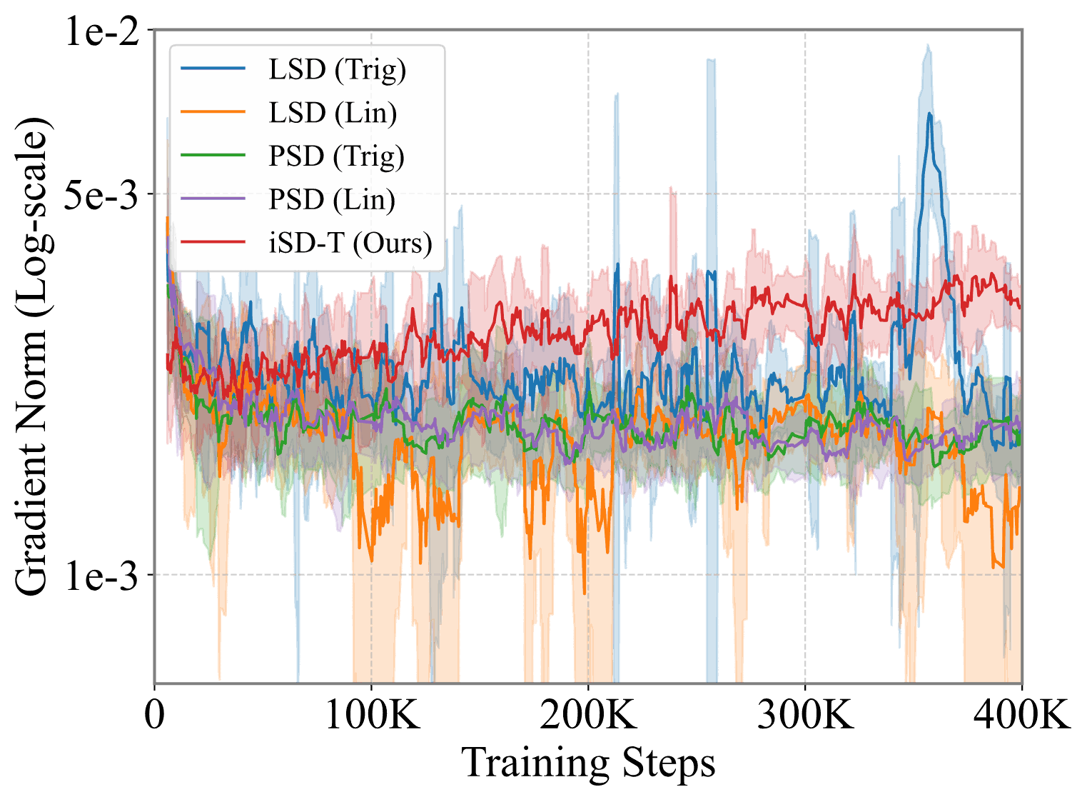
Gradient norms of self-distillation methods FIDs of self-distillation methods

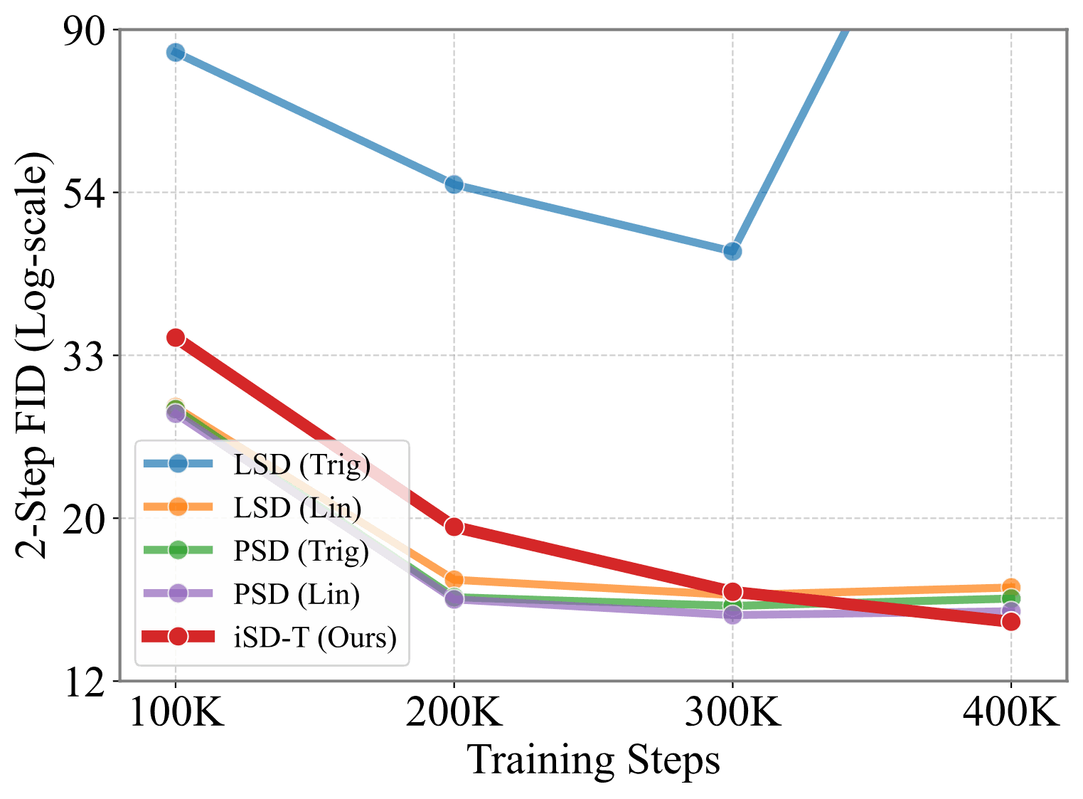
Figure 15. Training curves of self-distillation methods. All listed methods adopt Pre-CFG with \(\omega=5.0\). LSD shows more variable gradient norms than PSD and iSD-T, and its trigonometric variant diverges after a gradient spike around 350K training steps.

5.2 Implementation

Computing JVP. To align with the marginal velocity, \(dF_\theta/dt\) needs to follow \(dF_\theta/dt = \partial_tF_\theta + v_\theta\cdot \nabla_x F_\theta\). This can be implemented using standard JVP APIs with inputs \((x_t, t, s)\) and tangents \((v_\theta(x_t; t), 1, 0)\). This differs from prior work, which assumes tangents \((v_t(x_t|x), 1, 0)\). Alternatively, we can approximate it using a finite difference. Given a small step \(\epsilon\), we define displaced inputs as \(\hat x_{t\pm\epsilon} = x_t \pm \epsilon\cdot v_\theta\), and approximate \(dF_\theta/dt\approx [F_\theta(\hat x_{t+\epsilon}; t + \epsilon, s) - F_\theta(\hat x_{t-\epsilon}; t - \epsilon, s)] /(2\epsilon)\).

Classifier-free Guidance (CFG) is a widely used technique for improving diffusion models. However, since flow maps parameterize mappings rather than velocities, directly applying CFG does not guarantee mappings along the CFG velocity. We thus separate two extensions of iSD: Post-CFG and Pre-CFG. Post-CFG operates as a classical CFG:

\[\tilde f_\theta(x_t; t, s, c) = \nu^{-1}(A'_{t,s}x_t - A_{t,s} \tilde F_c),\quad \tilde F_c = F_\theta(x_t; t, s, \varnothing) + \omega(F_\theta(x_t; t, s, c) - F_\theta(x_t; t, s, \varnothing)).\]

Although this formulation is not guaranteed to follow the CFG velocity field, it can be readily applied after training. To ensure that the flow map follows the CFG field, we adopt a training-time CFG formulation (Geng et al., 2025), Pre-CFG. This incorporates CFG directly by replacing flow matching with:

\[\mathcal L_\mathrm{CFM}^\omega = \mathbb E\left[\left\|F_\theta(x_t; t, t, c) - \tilde v_t(x_t|x)\right\|^2_2\right],\qquad \tilde v_t(x_t|x) = F_\varnothing + \omega(v_t(x_t|x) - F_\varnothing),\]

where \(F_\varnothing = \operatorname{sg}[F_\theta(x_t; t, t, \varnothing)]\). We then train the flow map using the following objective:

\[\mathcal L_\mathrm{iSD\text{-}T} = \lambda_1\mathcal L_\mathrm{CFM}^\omega + \lambda_2\mathcal L_\mathrm{SD\text{-}R}.\]

This objective encourages the flow map to align with the ground-truth CFG velocity. We refer to this case as iSD-T (Training-time CFG). We adopt iSD-T for class-conditional settings and vanilla iSD for class-unconditional settings.

Algorithm 3: iSD-T Training
  1. Input: Noise distribution \(p_Z\), data distribution \(p_X\), model \(F_\theta\), learning rate \(\mu\), time distribution \(\tau\), adaptive weighting \((\eta, p)\), JVP approximation step size \(\epsilon\), Pre-CFG scale \(\omega\), class labels \(c\).
  2. repeat
  3. \(z \sim p_Z,\quad x \sim p_X,\quad t, s\gets \tau\)
  4. \(x_t\gets \alpha_t x + \sigma_t z,\quad v_t\gets \alpha'_tx + \sigma'_tz\)
  5. \(\tilde v_t \gets \omega v_t + (1-\omega)\operatorname{sg}[F_{\theta}(x_t; t, t, \varnothing)]\)
  6. \(F_{t,s}\gets F_\theta(x_t; t, s, c),\quad F_{t,t}\gets F_\theta(x_t; t, t, c)\)
  7. \(F'_{t,s}\gets \left[F_\theta(x_t + \epsilon F_{t,t}; t + \epsilon, s, c) - F_\theta(x_t - \epsilon F_{t,t}; t - \epsilon, s, c)\right] / (2\epsilon)\) ▷ JVP-Approx.
  8. \(F_\mathrm{tgt}\gets F_{t,s} + \left(A''_{t,s}x_t + A'_{t,s}(F_{t,t} - F_{t,s}) - A_{t,s}F'_{t,s}\right)\)
  9. \(\mathcal L \gets \lambda_1\|F_{t,t} - \tilde v_t\|^2_2 + \lambda_2\|F_{t,s} - \operatorname{sg}[F_\mathrm{tgt}]\|^2_2\) ▷ Optimization Target
  10. \(\theta\gets \theta-\mu\nabla_\theta \mathcal L\) ▷ Model Update
  11. until Convergence
Algorithm 2: iSD Sampling
  1. Input: Initial noise \(z\sim p_Z\), trained model \(F_\theta\), class labels \(c\), sampling time steps \(\{t_i\}_{i=1}^{N+1}\).
  2. \(x\gets z\)
  3. for \(i\gets 1\) to \(N\) do
  4. \(x \gets \nu^{-1}(A'_{t_i,t_{i+1}}x - A_{t_i,t_{i+1}}F_\theta(x; t_i, t_{i+1}, c))\)
  5. end for

Section 6

Experiments

To evaluate our method on image generation, we conduct experiments on the ImageNet-1K dataset. We use downsampled \(32\!\times\!32\!\times\!4\) latent variables from \(256\!\times\!256\) images encoded by a VAE, and adopt a DiT in BF16 precision. For unconditional settings, we validate our method on the CelebA-HQ dataset. We further evaluate our method on diffusion-based policy learning to assess the applicability beyond image generation.

6.1 Ablation Study

We conduct our ablation study on ImageNet-1K using DiT-B/4. The model is trained for 400K steps. We set \(\omega = 5.0\) for \(\mathcal L_\text{iSD-T}\) and use conditional velocity guidance for \(\mathcal L_\text{CT}\). All weights are randomly initialized. We measure the variance of quantitative results across five runs with different random initializations, and report mean values.

Table 3. Ablation study on ImageNet with DiT-B/4. 2-step evaluation results with standard deviations \(\sigma\).

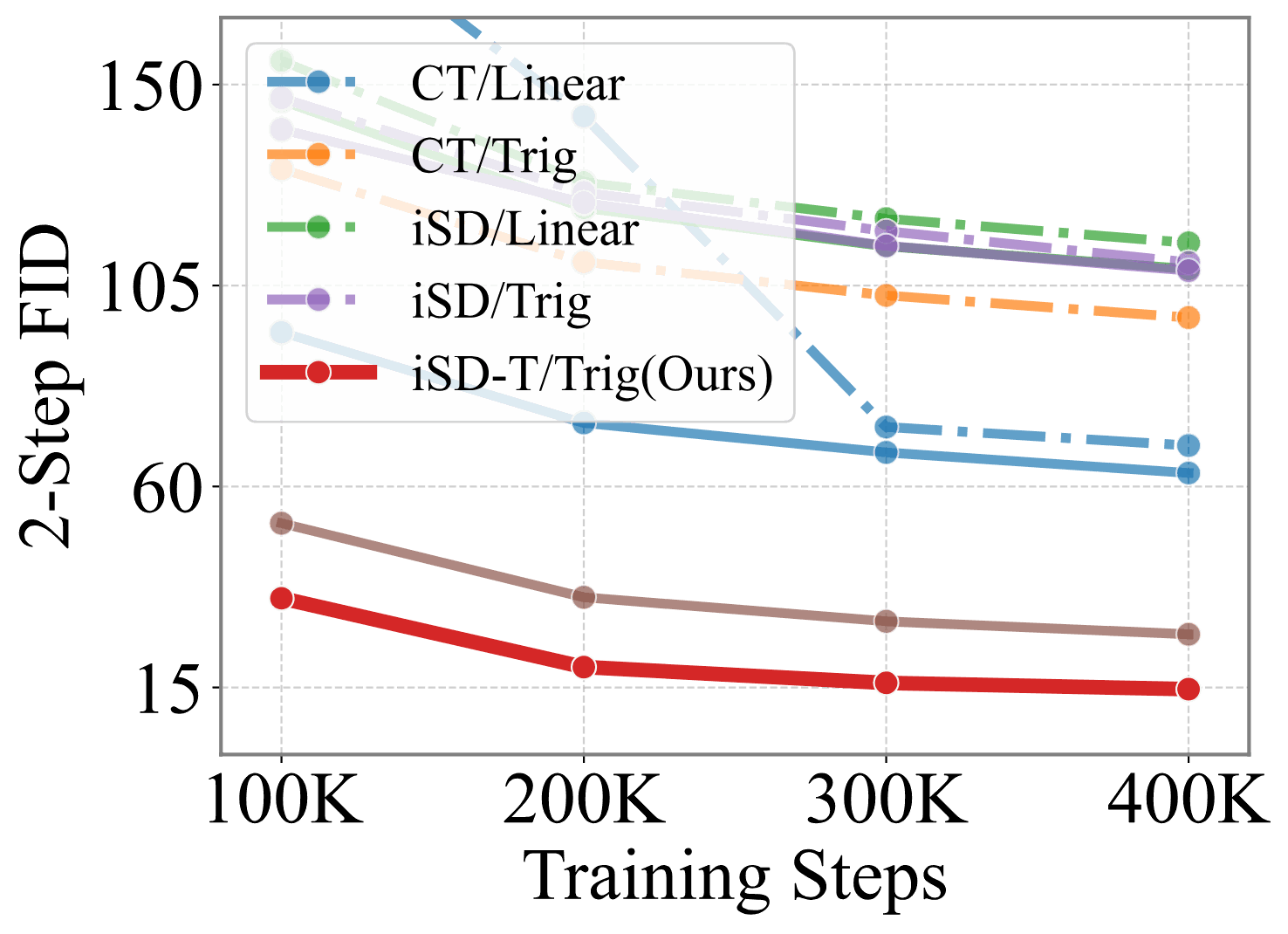
We begin with consistency training \(\mathcal L_\mathrm{CT}\) using linear interpolation. Joint training with flow matching improves results. Relaxing the time condition further improves results and reduces variance, which is consistent with our linearization cost hypothesis.

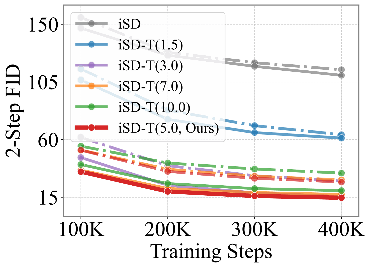
We observe that self-distillation alone underperforms, while incorporating Pre-CFG \(\mathcal L_\text{iSD-T}\) accelerates convergence, improves performance and reproducibility. One possible explanation is that vanilla iSD may trade the finite-batch residual for network approximation error, which can propagate to flow map training. Pre-CFG amplifies the class component and the flow map is trained along this sharpened field, whose task-relevant signal could become more prominent relative to the propagated approximation error.

FIDs over training steps across design choices(a) Design choices
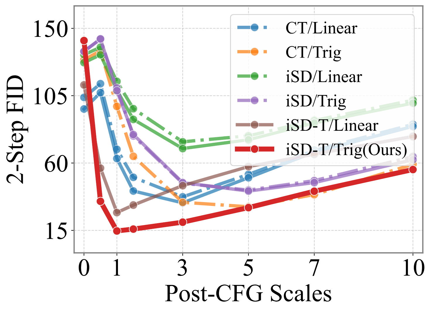
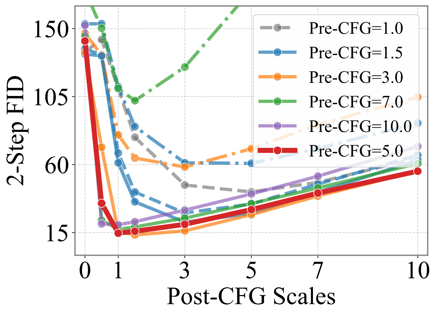
FIDs of Post-CFG over guidance scales(b) Post-CFG scales
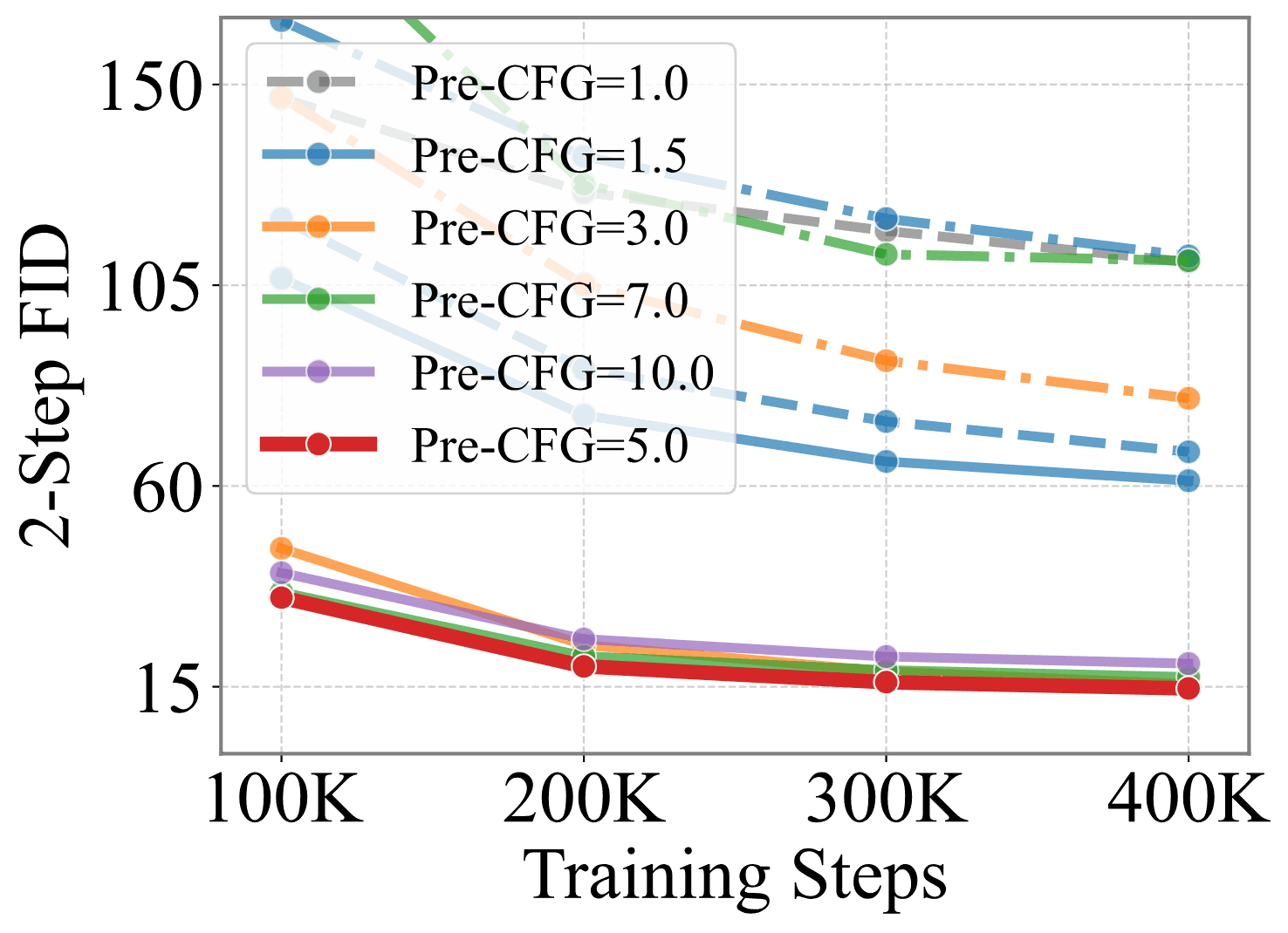
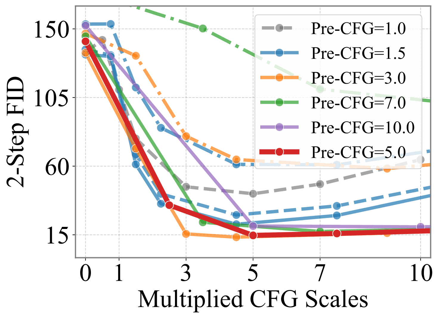
FIDs of Pre-CFG over training steps(c) Pre-CFG scales
Figure 5. Design choices. (a) FIDs over training steps. Solid lines indicate the JVP approximation, and dash-dot lines indicate the exact JVP. (b) FIDs of Post-CFG over guidance scales. (c) FIDs of Pre-CFG over training steps. Solid lines indicate trigonometric interpolation, and dash-dot lines indicate linear.
LossInterp.JVP1.03.05.07.0
\(\mathcal L_\text{CT}\)LinearExact69.1837.3952.4168.46
\(\mathcal L_\text{iSD}\)LinearExact114.5674.1778.2088.48
\(\mathcal L_\text{CT}\)LinearApprox.63.0233.4050.1867.27
\(\mathcal L_\text{iSD}\)LinearApprox.108.7069.6975.5386.72
\(\mathcal L_\text{iSD-T}\)LinearApprox.26.9144.9257.6065.92
\(\mathcal L_\text{iSD-T}\)TrigApprox.14.6220.4930.2141.15

Table 4. FIDs across design choices (2-step). The numbers in the header denote Post-CFG scales.

Interpolation. Linear interpolation tends to perform better under conditional velocity guidance, whereas trigonometric interpolation achieves lower FIDs under iSD-T. We observe varying performance across settings and tasks, leaving further analysis to future work.

JVP Operation. We observe that JVP approximation often yields better empirical results than exact computation. Under BF16 precision, it tends to be more robust, as the exact one is sensitive to numerical precision. The VRAM requirement of the training decreases from 25GB to 18GB on iSD-T, and the training speed improves from 1.48 steps/sec to 4.04 steps/sec on an A100 GPU.

Classifier-free Guidance. Incorporating Pre-CFG improves FIDs compared to the vanilla \(\mathcal L_\text{iSD}\). It also outperforms Post-CFG, which deviates from the intended CFG field, whereas Pre-CFG aligns the flow map with the CFG velocity during training. Combining both often degrades performance, as it results in applying the guidance twice, overly skewing the trajectory.

AppendixLoss curves, hyperparameters & Pre-CFG variants
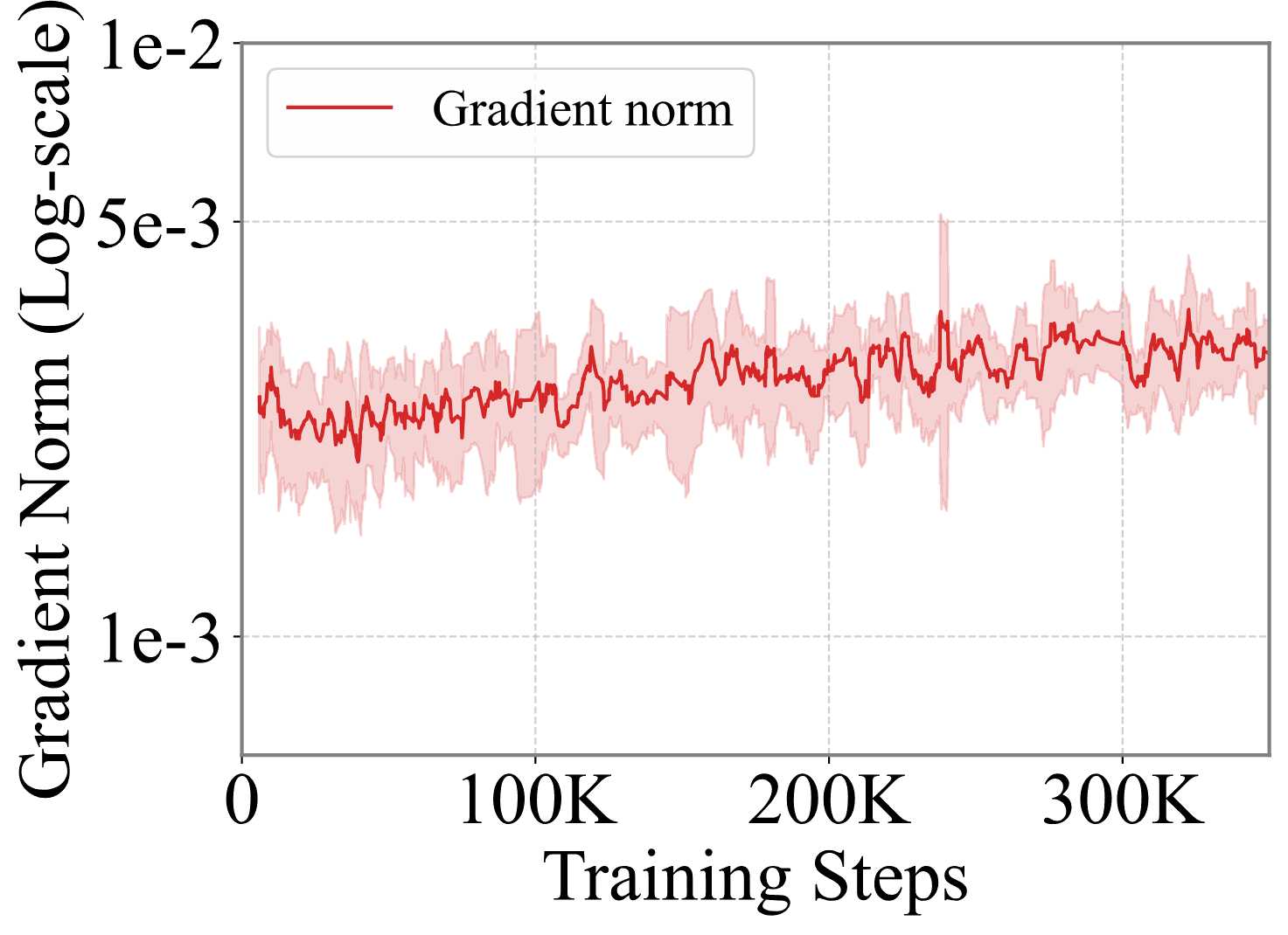
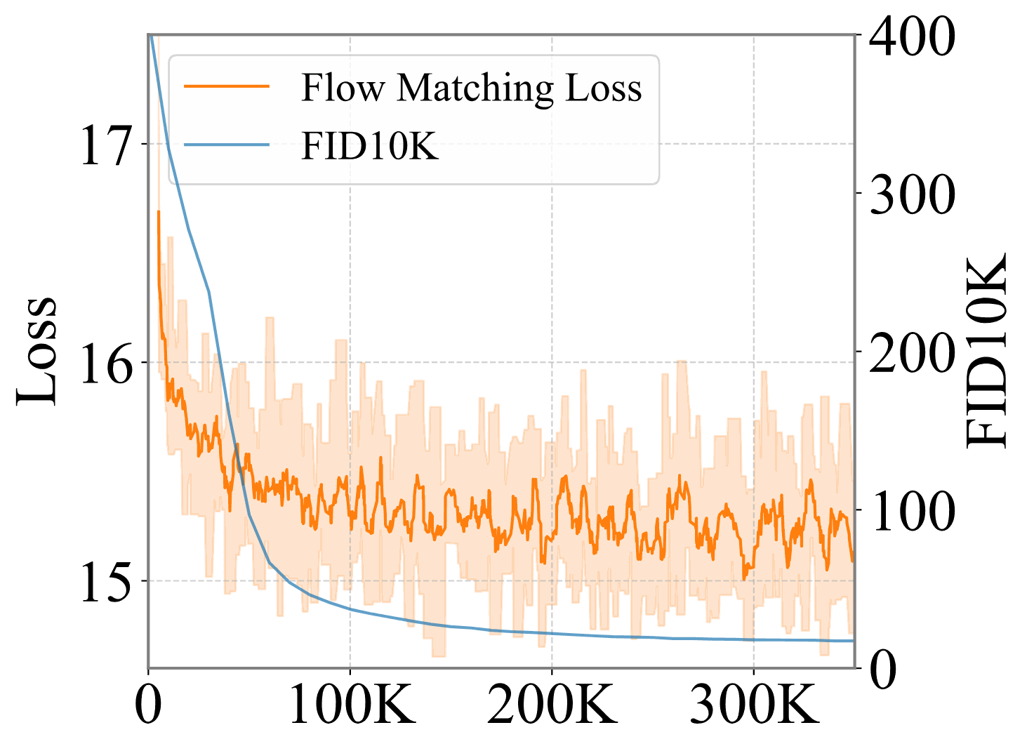
Gradient norm of iSD-T Flow matching loss of iSD-T SD-R loss of iSD-T

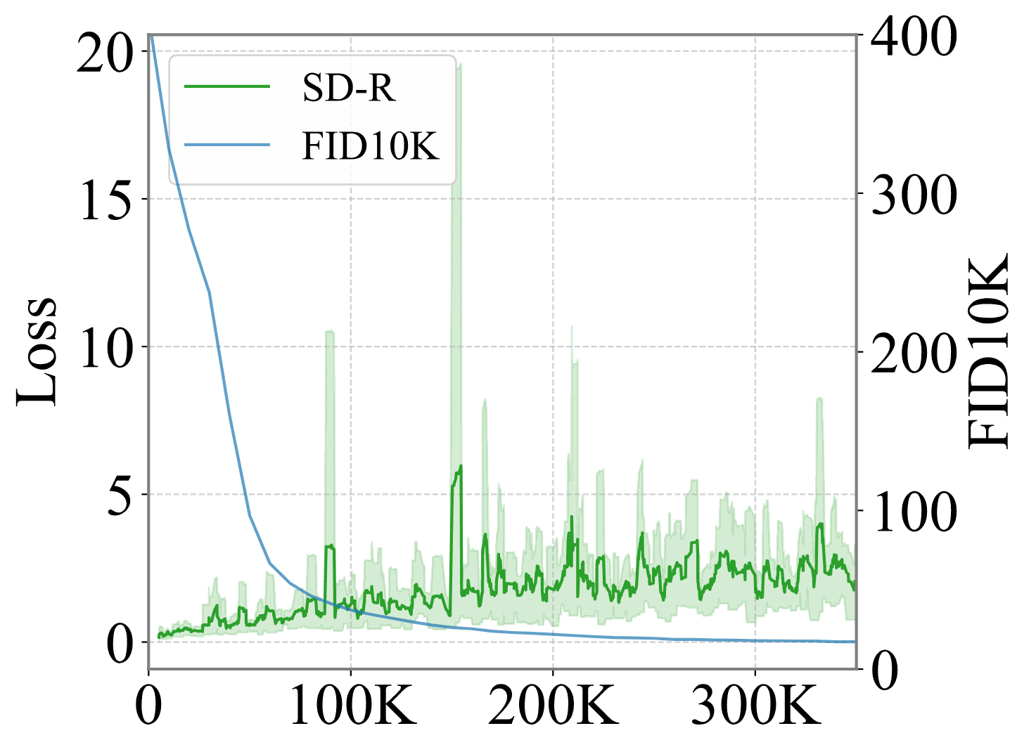
Figure 10. Gradient norm and loss curves of iSD-T compared to FID10K. FID and the flow matching loss decrease together over training, consistent with the role of velocity estimation in flow map training.

Table 5. Comparison on ImageNet with DiT-B/4. 2-step results with standard deviations \(\sigma\) under a controlled setup: the backbone, data, optimization, and training budgets are fixed, while the only difference lies in the training objective. Each method is evaluated using the CFG scale reported as optimal in its work.

Reproducibility. We examine the variance of quantitative results to assess reproducibility. Our iSD-T exhibits lower variance across runs compared to the baselines. From a performance perspective, we observe an FID gap with MeanFlow. Thus, a main advantage of iSD-T is more reproducible training outcomes with comparable sample quality.

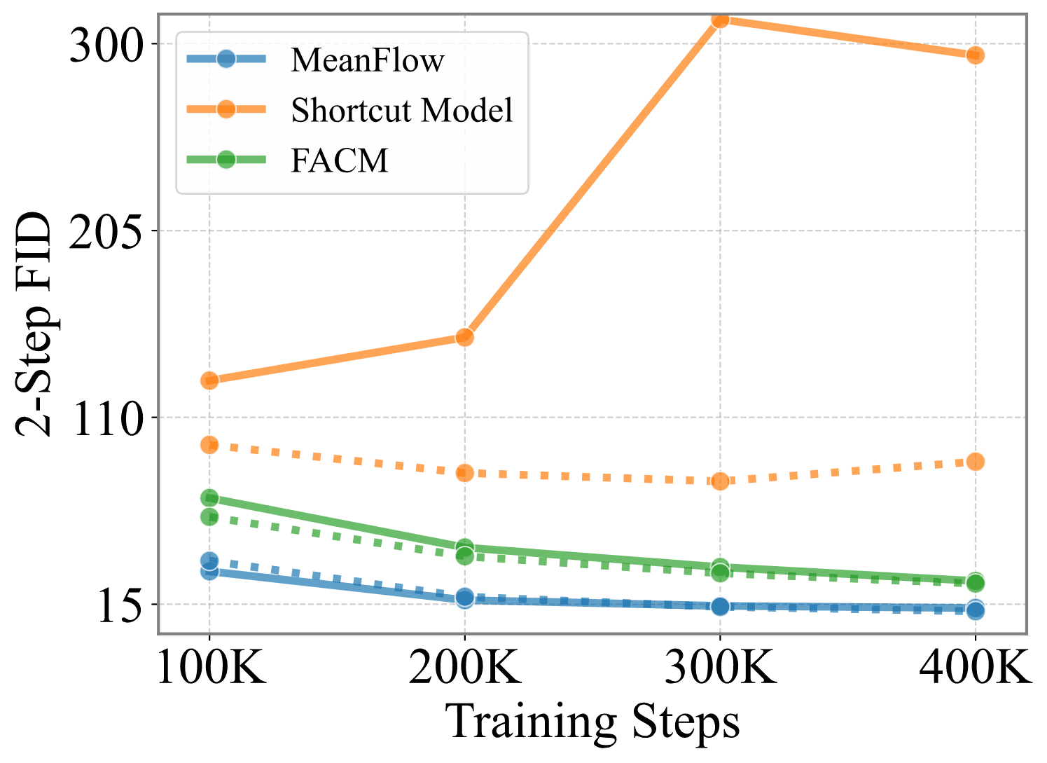
AppendixPrior work at \(\omega=5.0\)
FIDs of prior work at omega 5.0
CaseFID↓IS↑
MeanFlow13.12220.9
Shortcut Model128.76.57
FACM26.8585.05

Table 13. Comparison at \(\omega=5.0\).

Figure 13. FIDs on ImageNet. Solid lines indicate \(\omega=5.0\), and dotted lines indicate the \(\omega\) values in Table 5. Under this setting, the FIDs of MeanFlow and FACM increase relative to their reported scales. For the Shortcut Model, we did not observe stable convergence at larger guidance scales in our setup, and therefore report results using the recommended scale.

6.2 Comparison with Prior Work

Model4-FID↓128-FID↓
Distillation-based Methods
CD39.659.5
Reflow18.416.1
Training from Scratch
Flow Matching63.37.3
CT19.053.7
Shortcut Model13.86.9
iSD (Ours)11.37.1

Table 6. Comparison on unconditional CelebA-HQ.

ModelNFE↓FID↓
iCT220.3
Shortcut Model110.6
UCGM12.10
IMM27.77
MeanFlow22.20
FACM21.32
iSD-T (Ours, SD-VAE)22.76
iSD-T (Ours, VA-VAE)22.26

Table 7. Comparison on ImageNet-1K. iSD-T uses linear interpolation with a guidance scale of 5.0. This comparison assesses scalability under the combined setting, and the results reflect this configuration rather than the iSD objective alone.

Unconditional Generation. We compare our method with prior approaches on CelebA-HQ \(256\!\times\!256\) under a class-unconditional setting, using vanilla iSD without CFG. iSD achieves comparable performance in both few-step and multistep generation.

To examine scalability, we evaluate iSD-T with DiT-XL. iSD-T maintains stable training behavior and comparable sample quality at this scale. We note that achieving strong FID scores at this scale requires incorporating performance-oriented conditioning techniques, such as conditioning on a guidance scale or variations in latent representation. These choices are orthogonal to our analysis and are not required for stability.

Two-step ImageNet samples from iSD-T
Figure 6. 2-step results trained on ImageNet, iSD-T.

6.3 Diffusion-based Policy Learning

Transport
Push-T

Figure 7. Simulation results of the iSD policy with 2-NFE on Transport and Push-T tasks.

ModelNFE↓Push-TTransport
Diffusion Policy1000.951.00
10.120.00
Shortcut Model10.870.80
MeanFlow10.850.92
iSD (Ours)20.921.00
10.860.94

Table 8. Success rates (↑) of robotic control tasks.

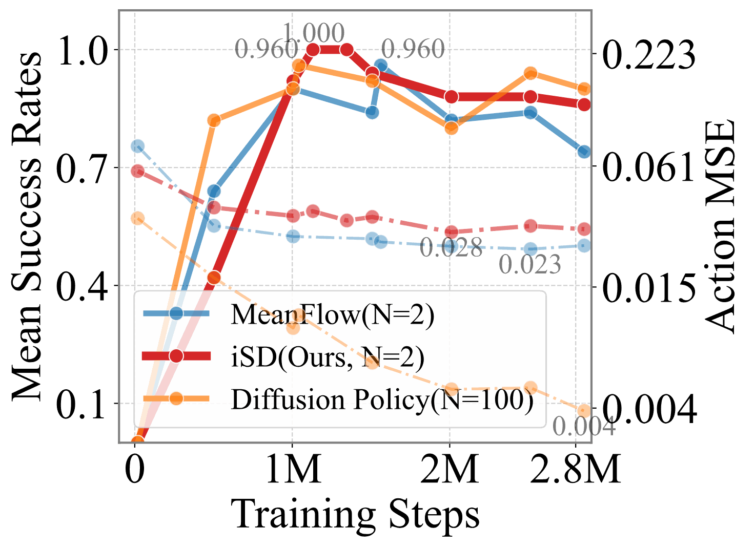
To assess the applicability of iSD beyond image generation, we adopt it as a diffusion policy objective in robotic control tasks. Experimental settings follow prior work on diffusion-based policies (Chi et al., 2023) for transformer and state-based architectures. This is intended to examine the applicability rather than to establish state-of-the-art results.

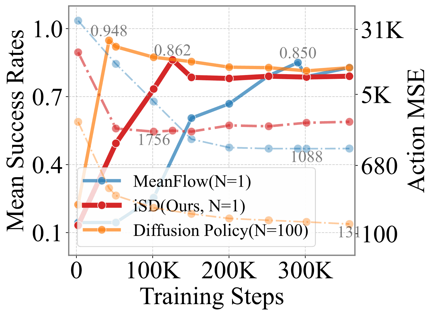
iSD with linear interpolation yields performance comparable to other few-step methods, under the same evaluation protocol. With 2-step sampling, iSD achieves success rates comparable to those of diffusion policies that require more sampling steps. These results indicate that iSD can serve as a few-step alternative to diffusion-based objectives in policy learning.

AppendixPolicy learning curves
Push-T success rate and action errorPush-T
Transport success rate and action errorTransport

Figure 16. Average success rates (solid lines) and action mean-squared errors (dash-dot lines) over training steps. Numeric entries indicate the optimal values across training steps.

Conclusion

In this work, we conducted a theoretical examination of consistency-based generative models from a flow map perspective, clarifying the sources of suboptimal convergence and training instability that can limit reproducibility. Building on these insights, we revisited self-distillation. To reduce its gradient norm problem, we empirically reformulated the self-distillation objective, yielding improved Self-Distillation (iSD). We further integrated training-time classifier-free guidance into iSD, yielding iSD-T with improved performance and reproducibility. Finally, we demonstrated that iSD is applicable to diffusion-based policy learning beyond image generation, without reliance on a pretrained diffusion model.

BibTeX

@article{kim2026stabilizing,
  title={Stabilizing Consistency Training: A Flow Map Analysis and Self-Distillation},
  author={YoungJoong Kim and Duhoe Kim and Woosung Kim and Jaesik Park},
  journal={Transactions on Machine Learning Research},
  issn={2835-8856},
  year={2026},
  url={https://openreview.net/forum?id=Qx2FrHDVzp},
  note={}
}